Homepage of Dionysus Birnbaum

Color Space

First, I want to point out that this isn't going to be a full article on persistent homology; this is just to give enough background on the little Python application I've got for you. If you already know a bit of homology, there's not much new, but hopefully the broad strokes I'll give are enough for anybody. Let's hop in; I'll provide the code at the end.

One of the ways you computer represents an image is as an array of RGB values; each pixel has some coordinate (the position in the array) and three whole numbers (R, G, B) between 0 and 255, representing the amount of red, green, and blue to emit and combine to make the color (additive color). Open up a paint application on your computer and go to the color swatches. You can play around, mixing red, green, and blue values. Maximum red and green with no blue gives yellow, maxing all three gives white, and so on.

Since any given color is just three numbers, we can distribute them spacially in three dimensions, by assigning (arbitrarily) the RGB values to xyz-coordinates. The R value says (for example) how far to move in the x-direction, G in the y-direction, and B in the z-direction. We can thereby convert a picture into a 3D scatter plot of points, based on their color. Take Van Gogh's "Wheatfield Under Thunderclouds" for example.

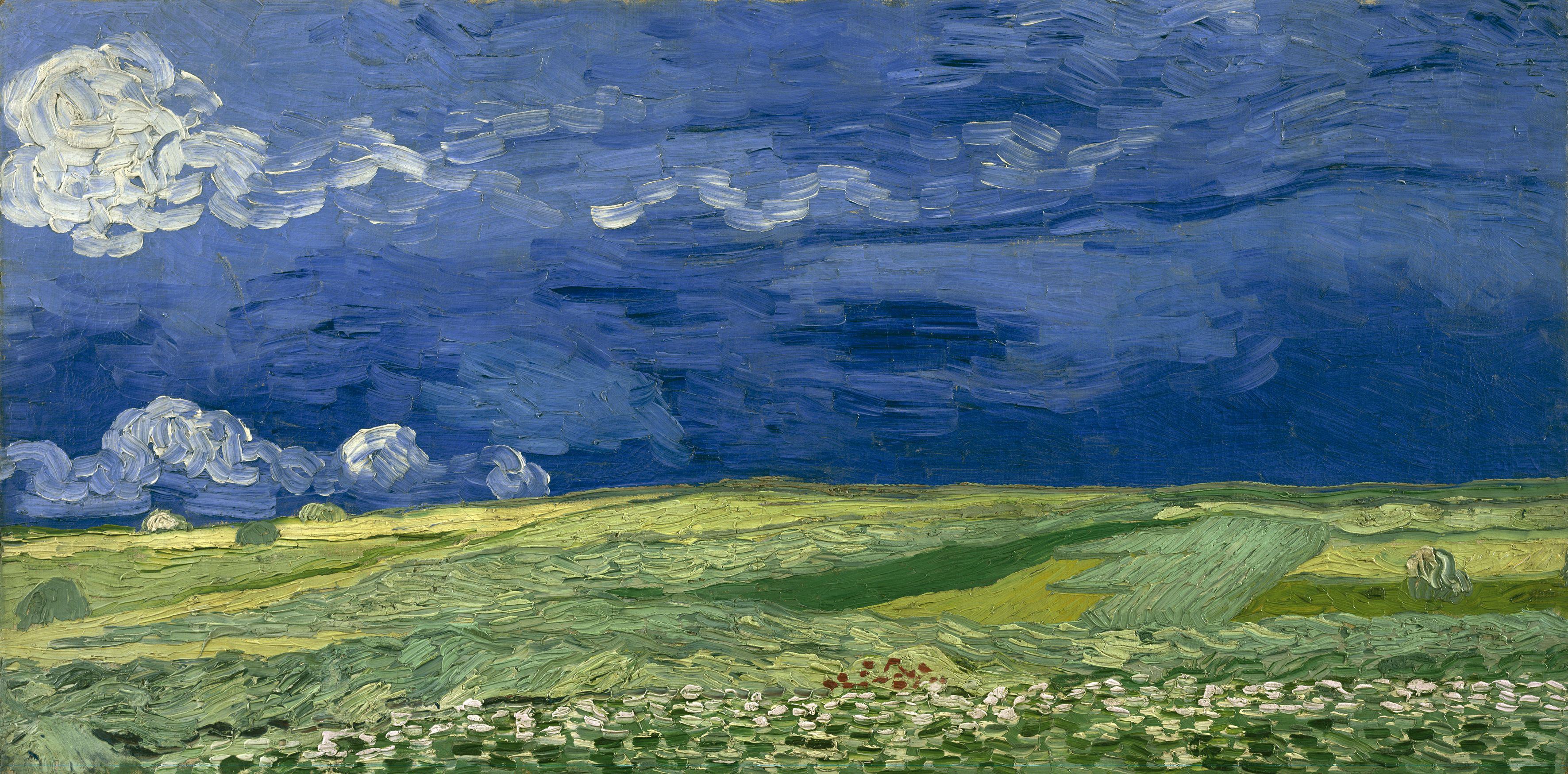
Visually, this painting is mostly two colors, so we would expect the color space to be, more or less, two clumps: one in the blue region of space and one in the green region of space. And, indeed, that is what we get.

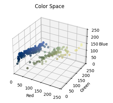
Wheatfield Under Thunderclouds Color Space

Once we have these points in space, we can start talking about topolgical properties. The most obvious one is the number of connected components, that is, the number of clusters the data points fall into. There are plenty of ways to do this, supervised and unsupervised: k-means, DBSCAN, etc. You can throw Python's scikit-learn at that and be on your merry way. Counting clusters like this is a special case of one of the key tools of algebraic topology: homology. Specifically, clustering is, more or less, computing the 0th homology of a space, simply the number of connected components. We need more tools, though, to talk through the "shape" in more detail.

Here's another Van Gogh example: "Wheatfield With Crows"

This painting shows a similar color space behavior: it is predominantly blue and yellow, so we get, more or less, two clusters. There's a little more red/orange and a little green, so depending on the cluster analysis you do, you could probably argue for one or two clusters. Two clusters if you say there is the blue/yellow split or one cluster if the little bit of red/orange and some of the outlying white connect the blue and yellow clumps. If we argue that there is only one component, there is another piece of shape information we can note: there may be one component, but it forms a loop.

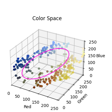
Counting the number of loops, the 1st homology after a sense, further distinguishes the shape of data. Compare a washer to a quarter, for example. Placing them on a grid and selecting out regular coordinates gives one cluster in both cases, but the washer has a hole or loop, while the quarter does not. The 1st homology detects that.

We can play this game in higher and higher dimensions, in fact. The only one we can still visualize, admittedly, is the 2nd homology, which describes a space being hollow, like a basketball or geode. What does a 3 or higher dimensional hollow look like? Tricky! But here's a color space example to show that off, too.

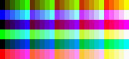
This picture is a little subtler and merits some explanation. The color space coordinate system is a 255 by 255 by 255 box. If you wanted the surface of the box, it would consist of all colors where one of the red, green, or blue component is fixed at 0 or 255. That is, you would allow all colors like (0, 5, 10) and (0, 50, 25) and (0, 255, 255); these are colors with red fixed at 0. We could fix green at 255, and allow all colors like (12, 255, 57) or (100, 255, 65) and so on. For each of the six possibilities (fixing R, G, or B at 0 or 255 for 3 times 2 equals 6 cases), I varied the other two components through {0, 50, 100, 150, 200, 250}, which gives an even spread of points on each face (admittedly with some .jpg compression muddying up the colors). The color space is given below, but it's not much to look at, as the points are all on the "surface" of the cube, blocking out view of the hollow insider, where there are no points.

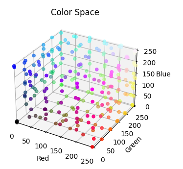
This color space ought to have one cluster (0th homology) since the points are evenly distributed on the surface of a cube; no way to reasonably split them apart. It has zero loops (1st homology) since there's nothing you could pass a string through and tie off. And finally it has one hollow (2nd homology) consisting of the inside of the box, separated from the outside.

Now, to make this a tad more rigourous, I'll sketch out the idea behind persistent homology, what's actually being computed. Given one of these color spaces, consisting of a cloud of points in three-dimensions, I want you to imaging a ball around each point, that steadily inflates. At the start, each ball only covers its own point so as far as homology is concerned, we have one cluster for each point, no loops, no hollows, nothing beyond the cluster for each point. But as the balls inflate, they start merging together, which combines clusters. Clusters start to die off and, potentially, loops or hollows start to form (picture the surface of the box covered in dollops of spray-foam insulation; as the foam inflates, it merges together, until the box is covered). As the balls grow larger and larger, eventually everything is mashed together until there is only one cluster and, again, no loops or hollows.

Homology does a pile of linear algebra to describe how many clusters there are, how many loops there are (as well as where the loops are in terms of balls-arond-points), how many hollows, etc. The "persistent" side is describing how, at certain sizes loops, hollows, etc. form (are "born") and then, as the balls grow larger, "die" off. If a loop or hollow has a long lifetime ("persistent") we assume it represents some intrinsic, topological information about the data.

Let's see that play out. Here's "Wheatfield Under Thunderclouds" again:

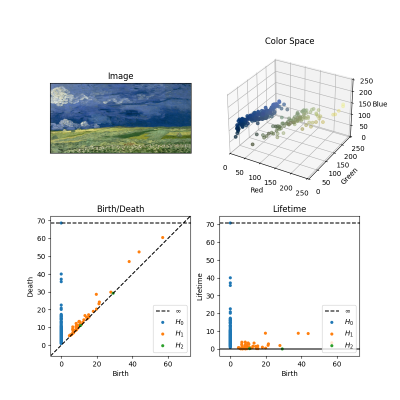
Without a bit of practice, it's difficult to read these plots, but let me run through the highlights. Each component of the homology has an xy-coordinate, describing what radius it was born at and what radius it died at. Nothing ever dies before it is born, so there is nothing under the line y=x (anything under the line y=x would say the radius at which it died was smaller than the radius at which it was born). The higher above the y=x line on the Birth/Death chart (or equivalent the higher up on the Lifetime) chart, the longer that component persisted. We can see, for example, there are no particularly long lasting components of the 1st or 2nd homology (yellow and green, respectively).

And now "Wheatfield With Crows"

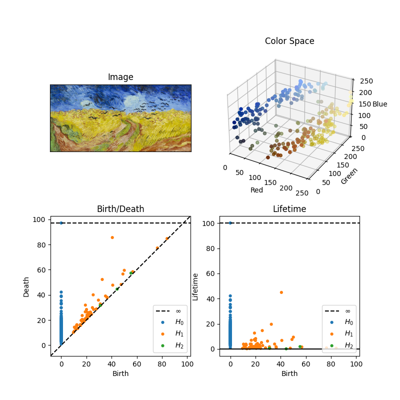
With this, we still don't have much lasting for the 2nd homology, but at a birth radius of about 40, we have a component of the 1st homology with a very long lifespan! From a radius of 40 to a radius of about 80, there is a loop.

And now the custom gradient:

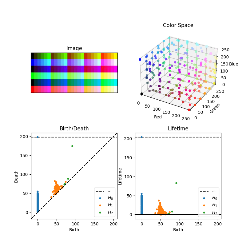
Again, nothing too, too lasting for the 1st homology, but now we have a persistent element of the second homology. (And a very dense die-off of the 0th homology; we very quickly detect that there is really only one cluster.)

Finally, because I've somewhat neglected the 0th homology on these examples, here's a quick one which shows that, yes, the 0th homology is describing the number of clusters (albeit in a way that is hard to read from the birth/death). Presenting, Piet Mondrian's "Composition II in Red, Blue, and Yellow":

Composition II in Red, Blue, and Yellow Color Space

There is essentially nothing for the 1st and 2nd homology, while we see a very spread out birth/death for the 0th homology, for a large number of distinct clusters.

Okay. With all that said, here are the files.